Overview
The Dynamic Stochastic General Equilibrium (DSGE) model is used to model the joint behavior of aggregate time series in macroeconomics, such as inflation, interest rates, and unemployment. DSGE is used to analyze policies, for example, to answer this question: What effect does a sudden rise in interest rates have on inflation and output? To answer this question, we need a model of the relationship between interest rates, inflation, and output. Because the multiple time series of the DSGE model is closely related to economic theory, it can be distinguished from other models. Macroeconomic theory consists of decision-making model equations of families, companies, decision makers, and other agents that form the DSGE model. Since the DSGE model is theoretically derived, its parameters can be explained directly from a theoretical perspective.
In this article, I built a small DSGE model similar to the monetary policy analysis model. It will demonstrate how to use the new dsge command in Stata15 to estimate the parameters of this model. Then, use the currency contraction policy to impact the model and plot the response curve of the model variable to the impact.
Small DSGE model
A DSGE model begins with a description of the economic sector. The models described here are related to models developed in Clarida, GalÃ, Gertler (1999) and Woodford (2003). It is a smaller version of the various models used by central banks and academia for monetary policy analysis. The model has three departments: family, company and central bank.
Household consumption output. Their decision is summarised by an output demand equation that links current output demand to expected future output demand and real interest rate.
Manufacturers set prices and yields to meet the set price requirements. Their decisions are summarised by a pricing equation that links current inflation (ie, price changes) to expected future inflation and current demand. The extent to which inflation depends on output demand plays a key role in the model.
The central bank sets a nominal interest rate in response to inflation. When inflation rises, the central bank raises interest rates and lowers interest rates as inflation falls.
The model can be summarized into three equations.
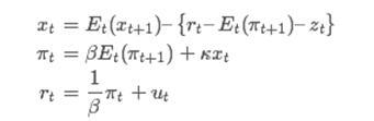
The variable xt represents the output gap. The output gap measures the difference between output and long-term natural value. The symbol Et(xt+1) specifies the expected information for the output gap during t+1, the nominal interest rate is rt, and the inflation rate is πt. Equation (1) indicates that the output gap is positively correlated with the expected future output gap Et(xt+1) and negatively correlated with the {rt- Et(πt+1)-zt} interest rate gap. The second equation is the company's pricing equation; it links inflation to the expected future inflation and output gap. The parameter κ determines the extent to which inflation depends on the output gap. Finally, the third equation summarizes the behavior of the central bank; it links interest rates to inflation and other factors, collectively referred to as ut.
The endogenous variables xt, πt and rt are driven by two exogenous variables zt and ut. In theory, zt is the natural interest rate. If the real interest rate is equal to the natural rate and is expected to remain unchanged in the future, then the output gap is zero. The exogenous variable ut captures all changes in the interest rate generated by factors other than the inflationary movement. It is sometimes referred to as an unexpected component of monetary policy.
These two exogenous variables are modeled as a first-order autoregressive process.
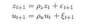
It is customary.
In jargon, endogenous variables are called control variables, and exogenous variables are called state variables. In one cycle, the value of the control variable is determined by the system of equations. Control variables can be observed or observed. State variables are fixed at the beginning of a cycle and are not observed. The equations determine the state variable values ​​of the state variables in a future period.
We hope to use this model to answer policy questions. What is the impact on the model variables when the central bank raises interest rates unexpectedly? The answer to this question is the effect of imposing a pulse ξt and tracking pulse time.
Before performing a strategy analysis, we must assign values ​​to the parameters of the model. We will use US inflation data and use
The dsge interest rate in Stata is used to evaluate the parameters of the above model.
Specify a DSGE model
I use the US interest rate and inflation rate data to fit the model. In the DSGE model, there are many observable control variables that can impact the model. Since the model has two shocks, we have two observable control variables. The variables in a linear DSGE model are stationary, measured from steady-state deviations. In practice, this means that the data must meet previous estimates. Dsge will delete your average model.
The data I used in usmacro2 is from the St. Louis database of the Federal Reserve Bank.

To assign a model to Stata, type the formula using a replaceable expression.
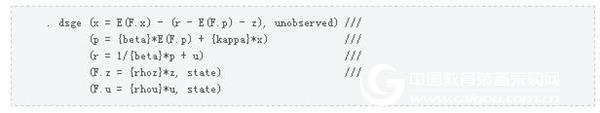
The rules of the equation are similar to the specific alternative expressions of the work of other Stata commands. Each equation is enclosed in parentheses. Parameters are enclosed in braces to distinguish them from variables. Expected values ​​for future variables appear in the E () operator. The variable appears to the left of the equation. In addition, each variable in the model appears to the left of an equation. Variables can be observed (as variables in the dataset) or not observed. Since the state variable is fixed during the current cycle, the equation of the state variable indicates how the one-step pre-value of the state variable depends on the current state variable and may also depend on the current control variable.
Evaluate the model parameters to give us an output table:
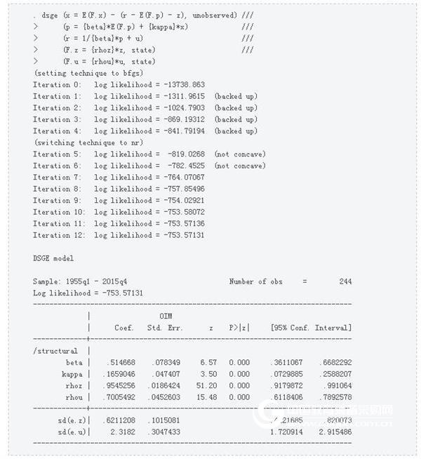
The key parameter is {kappa}, which is estimated to be positive. This parameter is related to potential price conflicts in the model. Its explanation is that if we expect the inflation rate to remain unchanged in the future, a percentage point of the output gap will lead to an inflation rate increase of 0.17 percentage points.
The parameter β is estimated to be around 0.5, which means that the inflation coefficient in the interest rate equation is about 2. As a result, the central bank doubled interest rates based on changes in inflation. This parameter is discussed in much in the monetary economics literature, and its estimate is around 1.5. The values ​​found here are comparable to these estimates. Both state variables zt and ut are estimated to be persistent, with autoregressive coefficients of 0.95 and 0.7, respectively.
Pulse-reaction
We can now use the model to answer questions. One question that the model can answer is: What is the impact of unexpected changes in interest rates on inflation and output gaps? Unexpected changes in interest rates are considered to be an impact on the ut equation. In the language of the model, this shock reflects the contraction of monetary policy.
In (5): (1, 0, 0, 0, 0, ...), one pulse is a series of values ​​for the impact ξ. Then it hits the state variable of the model, causing u to grow. There, the growth of u leads to changes in the control variables of all models. A pulse-response function tracks the impact of the impact on the model variables, taking into account the interrelationships between all the variables present in the model equations.
We type three commands to build and draw an IRF. The irf set sets the IRF file and retains the impulse response file. Irf create creates a set of impulse response files in the IRF file.

By saving the impulse response file, we can draw them:
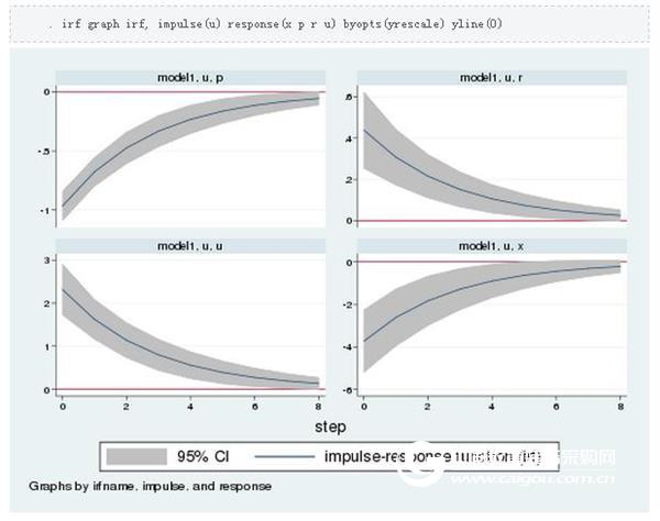
The impulse response map maps the response of the model variable to a standard deviation shock. Each panel is a variable response to the shock. Since the impact, the horizontal axis measures the time after the impact, and the vertical axis measures the time from the long-term value. The lower left panel shows the response of the currency status variable ut. The remaining three panels show the reaction of inflation, interest rates and output gaps. Inflation is the panel on the upper left, which is affected by the impact. The interest rate response in the upper right panel is the weighted sum of inflation and currency shock – response. Interest rates have risen by about half a percentage point. Finally, the output gap has fallen. Therefore, the model predicts that after the monetary tightening policy, the economy will enter a recession. Over time, the effects of the shock dissipated and all variables returned to their long-term value.
to sum up
In this article, we created a small DSGE model that describes how to use the estimated dsge model parameters. Then, it demonstrates how to create and interpret an impulse response function.
The Chinese Science Software Network has compiled a tutorial on the use of the Stata software series. For other articles, please log in to view.
Mobile Green Screen,Foldable Green Screen,Portable Foldable Green Screen,Portable Foldable Mobile Green Screen
Dongguan Aoxing Audio Visual Equipment CO.,Ltd , https://www.aoxing-whiteboard.com